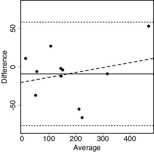
R code used to produce the graph shown below.

hplc <- c(139, 120, 143, 496, 149, 52, 184, 190, 32, 312, 19) 
gcms <- c(151, 93, 145, 443, 153, 58, 239, 256, 69, 321, 8) 
average <- (hplc + gcms)/2           # Compute average 
dif <- (hplc - gcms)                 # and difference 
plot(average, dif, ylim=c(-80,80),   # Plot diff vs average 
     xlab="Average", ylab="Difference", cex=mycex) 
limit <- qnorm(.975) 
# Add average bias and 95% limits of agreement 
abline(h=mean(dif)+c(-limit,0,limit)*sd(dif),lty=c(3,1,3)) 
# Add line showing bias as function of magnitude 
abline(lm(dif~average), lty=2)